Data Analysis Bootcamp: Lecture 0
Table of contents
- Introduction
- Prerequisites
- Toolbox
- Exercise 0: My first ROOT macro
- Interlude: Is this good enough? A first look into p-values
- A signal + background problem
Prerequisites
- A computer
- Not being afraid of using it: physicists are famous for writing horrible code, you cannot but improve our reputation among developers.
- Not being afraid to ask: learning physics takes long enough, there is little time left to learn programming in your studies. It’s ok if you have no idea how to do something, but rest assured there is a high chance you can do it. You just have to ask the right questions to the right people.
- Open mind: in general, consider the realm of numerical methods as tools to expand your reach as a physicist.
Toolbox
- Text editor: take some time to explore few options, and then some more time to learn how to exploit it to your best for coding. Few features can be a game changer for your productivity
- git: We are using git to distribute the code we develop in this workshop. It’s the standard for collaborative development and distribution. You may want to consider using this course as an opportunity to start practicing the dark arts of repository management.
- ROOT: “Community standard” for data analysis in particle and nuclear physics. Being a C++ based package it may be a bit less handy than some alternatives, but it comes with 30 years of people asking on the internet how to fill and fit a histogram with it.
Exercise 0: My first ROOT macro
The simplest way of using ROOT is to write a macro, a script that is executed by ROOT’s interpreter. ROOT macros are typically slightly less efficient than compiled code, but arguably easier to write and debug.
Step 1: Building a histogram
Let’s start with a simple example: reading a histogram from a txt file and plotting it.
#include <iostream>
#include <fstream>
#include <sstream>
#include "TFile.h"
#include "TCanvas.h"
#include "TH1D.h"

int MyFirstRootMacro(const TString filename = "test_data.txt")
{
  // --------------------------------------------------------------------
  // Build the data histogram
  // --------------------------------------------------------------------

  // Open and read the input file in a stream
  std::ifstream inputfile;
  inputfile.open(filename);
  if (!inputfile.is_open()) {
    std::cerr << "Error: file " << filename << " not found." << std::endl;
    return 1;
  }

  // Create a histogram to store the data
  TH1D* h = new TH1D("h", "My first histogram;Channel;Counts", 2048, 0, 2048);

  std::string line;
  std::getline(inputfile, line); // Skip the header

  // Read the data from the file
  int channel = 0;
  double counts = 666;

  while ( std::getline(inputfile, line) ) {
    std::istringstream iss(line);
    // Read the data from the file
    iss >> channel >> counts;
    // Set counts in channel
    h->SetBinContent(channel, counts);
  }

  // Draw the histogram
  TCanvas* c = new TCanvas("c", "My first canvas", 800, 600);
  h->Draw();

  return 0;
}
Notes: the function uses the same name as the macro file as it is automatically executed when passing the macro file to ROOT at startup as in
$ root MyFirstRootMacro.C
Let’s spice things up a bit by using a including other functions to be called by the main one.
...
/**
 * @brief A function that checks the bin errors of a histogram
 *
 * @param h input histogram
 * @return true if all bin errors are correct, false otherwise
 */
bool check_errors(const TH1D* h)
{
  bool bin_check = true;
  for (int i = 1; i <= h->GetNbinsX(); i++) {
    const double err = h->GetBinError(i);
    const double content = h->GetBinContent(i);
    if ( err != sqrt(content) ) {
      std::cerr << "Error: bin " << i << " has an error of " << err << " and a content of " << content << std::endl;
      bin_check = false;
    }
  }
  return bin_check;
}

/**
 * @brief Fill a histogram with data from a text file
 *
 * @param h target histogram
 * @param filename txt file path
 * @return 0 if successful
 */
int fill_hist_from_txt(TH1D* h, const TString filename);

int MyFirstRootMacro(const TString filename = "test_data.txt")
{
  // Create a histogram to store the data
  TH1D* h = new TH1D("h", "My first histogram;Channel;Counts", 2048, 0, 2048);
  // Fill the histogram with data from the file
  int fill_status = fill_hist_from_txt(h, filename);
  if (fill_status != 0) {
    std::cout << "Error: fill_hist_from_txt failed with status " << fill_status << std::endl;
    return 1;
  }

  // Check bin errors
  bool bin_check = check_errors(h);

  // Draw the histogram
  TCanvas* c = new TCanvas("c", "My first canvas", 800, 600);
  h->Draw();

  return 0;
}

// One must always define the functions before calling them, but the
// actual implementation can be placed at the end of the file
int fill_hist_from_txt(TH1D* h, const TString filename)
{
  // Open and read the input file in a stream
  std::ifstream inputfile;
  inputfile.open(filename);
  if (!inputfile.is_open()) {
    std::cerr << "Error: file " << filename << " not found." << std::endl;
    return 1;
  }
  std::string line;
  std::getline(inputfile, line); // Skip the header

  // Read the data from the file
  int channel = 0;
  double counts = 666;
  while ( std::getline(inputfile, line) ) {
    // Read the data from the file
    std::istringstream sstream(line);
    sstream >> channel >> counts;
    h->SetBinContent(channel, counts);
  }
  // Close the input file
  inputfile.close();
  return 0;
}
Step 2: Fitting the histogram
We can now define a model to fit our data. Analytical functions in ROOT are represented by the TF1 class. Note that you can construct a TF1 object in many different ways (see TF1 documentation). Here a non-exhaustive list of possible ways to define a TF1 object:
// Inline expression with built-in functions
f = new TF1("f", "gaus", 0, 2048);
// Inline expression with parameters
f = new TF1("f", "[0]*exp(-0.5*TMath::Sq((x-[1])/[2]))", 0, 2048);
// General C function with parameters [e.g, double my_c_gaus(double* x, double* par)]
f = new TF1("f", my_c_gaus, 0, 2048, 3);
// Lambda expression with parameters
f = new TF1("f", [](double* x, double* par) {
        double constant = par[0];
        double mean = par[1];
        double sigma = par[2];
        double y = constant * exp(-0.5 * TMath::Sq((x[0] - mean) / sigma));
        return y;
        }, 0, 2048, 3);
Let’s plug one of these into our macro:
...

int MyFirstRootMacro(const TString filename = "test_data.txt")
{
  // --------------------------------------------------------------------
  // Build the data histogram
  // --------------------------------------------------------------------

  // Create a histogram to store the data
  TH1D* h = new TH1D("h", "My first histogram;Channel;Counts", 2048, 0, 2048);

  // Fill the histogram with data from the file
  int fill_status = fill_hist_from_txt(h, filename);
  if (fill_status != 0) {
    std::cout << "Error: fill_hist_from_txt failed with status " << fill_status << std::endl;
    return 1;
  }

  // Check bin errors
  bool bin_check = check_errors(h);

  // Draw the histogram
  TCanvas* c = new TCanvas("c", "My first canvas", 800, 600);
  h->Draw();

  // --------------------------------------------------------------------
  // Define model
  // --------------------------------------------------------------------
  // Create a fit model
  TF1* f = new TF1("f", "gaus", 0, 2048); // Built-in Gaussian function

  f->SetParName(0, "Constant");
  f->SetParName(1, "#mu");
  f->SetParName(2, "#sigma");

  // Initialize the parameters
  f->SetParameter(0, h->GetMaximum());
  f->SetParameter(1, h->GetMean());
  f->SetParameter(2, h->GetRMS());

  // --------------------------------------------------------------------
  // Fit the data
  // --------------------------------------------------------------------
  // Set the fit range
  double xmin = h->GetMean() - 2*h->GetRMS();
  double xmax = h->GetMean() + 2*h->GetRMS();

  // Fit the histogram
  TFitResultPtr result = h->Fit(f, "S", "", xmin, xmax);

  // retrieve the χ² value and the ndf
  const double chi2 = result->Chi2();
  const double ndf = result->Ndf();

  // compute the p-value
  double p_value = TMath::Prob(chi2, ndf);
  std::cout << "p-value: " << p_value << std::endl;

  if (p_value < 0.05) {
    std::cout << "Warning: the p-value is less than 0.05" << std::endl;
    return 1;
  }

  return 0;
}
Interlude: Is this good enough? A first look into p-values
What any physicist would do after fitting a histogram is to check the goodness of the fit, typically by looking at the χ²/ndf value. How did we end up here?
By default, the Fit method in ROOT minimizes a χ² function defined as:
where \(h_i\) is the observed number of counts in the bin \(i\), \(\boldsymbol{\theta}\) are the model’s parameters, and \(f(x_i|\boldsymbol{\theta})\) is the model prediction for the bin \(i\).
This function happens to be a limit case of the more general likelihood function, which is the product of Poisson probabilities for each bin (Poissonian Binned Likelihood):
\[\mathcal{L}(\{h\}|\boldsymbol{\theta}) = \prod_{i=1}^{N} \frac{e^{-\lambda_i} \lambda^{h_i}}{h_i!} \quad \text{with } \lambda_i = f(x_i|\boldsymbol{\theta})\]in the limit of a large number of counts per bin, the Poisson distribution can be approximated by a Gaussian distribution with mean \(\lambda_i\) and variance \(\lambda_i\):
\[\mathcal{L}(\{h\}|\boldsymbol{\theta}) \approx \prod_{i=1}^{N} \frac{1}{\sqrt{2\pi\lambda_i}} e^{-\frac{(h_i - \lambda_i)^2}{2\lambda_i}}\]By taking the negative logarithm of the likelihood function, one can show that the minimizing the χ² function is equivalent to maximizing the likelihood function. (note that in this limit case we obtain the Pearson’s definition of the χ², which is the one used in the ROOT Fit method. One should pass the option P to use it instead).
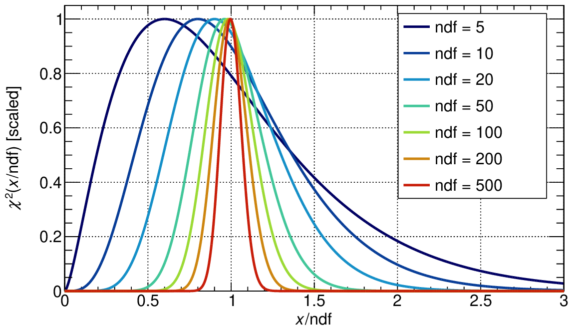
A common practice among physicists is to consider a fit “good” if the χ²/ndf is close to 1, but keep in mind that how close depends on the number of degrees of freedom.

A more quantitive way to assess the goodness of the fit is to compute the p-value, which is the probability of observing a χ² value as extreme as the one obtained from the fit.
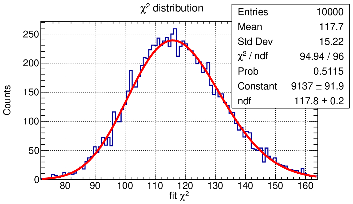
But what does it mean in practice? What distribution do you expect for p-values?
Check out this other macro: lecture_0/ex0/p_value_test.C
In this macro we simulate multiple “experiments” and fit the data with a Gaussian model, observing the distribution of the fit results, of the fit χ² and of the p-value.

A signal + background problem
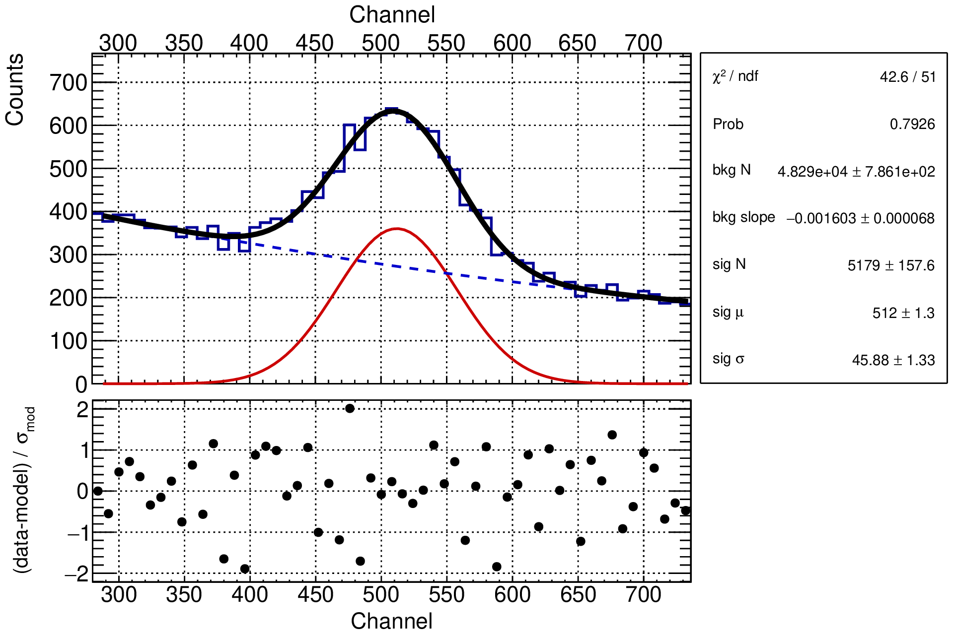
Let’s now consider a textbook case: a signal + background problem. We will generate a dataset with a Gaussian signal and an exponential background, and try to fit it with a model that includes both components.
The example macro is available at lecture_0/ex1/l0ex1_sb_single.cc.
To make it easier to change the statistics of the dataset, we will define the signal and background rates and multiply them by the exposure time to get the number of events.
Our parameters of interests are the ones controlling the signal and background shapes, and the number of signal and background events. Let’s make use of the lambda-expression constructor of the TF1 class to define the signal and background PDFs and then combine them into a model PDF.
// --------------------------------------------------------------------
// Define model for the signal, background and data
// --------------------------------------------------------------------
TF1* fSignal = new TF1("signal",
    [bin_width](double* x, double* p)
    {return bin_width*p[0]*TMath::Gaus(x[0], p[1], p[2], true);},
    0, 2048, 3);

TF1* fBackground = new TF1("background",
    [bin_width](double* x, double* p)
    {return -bin_width*p[0]*p[1]*exp(x[0]*p[1]);},
    0, 2048, 2);

TF1* fModel = new TF1("fModel",
    [bin_width, fBackground, fSignal](double* x, double* p) {
      fBackground->SetParameters(p[0], p[1]);
      fSignal->SetParameters(p[2], p[3], p[4]);
      double y = fBackground->Eval(x[0]) + fSignal->Eval(x[0]);
      return y;
    },
    0, 2048, 5);
Another way to scrutinize the fit result is to look at the residuals of the fit, which are the difference between the data and the model divided by the uncertainty. You can write a simple function to compute them:
TH1D* make_residuals(const TH1D* h_data, const TF1* fModel, const double xmin, const double xmax)
{
  TH1D* h_res = static_cast<TH1D*>(h_data->Clone("h_res"));
  h_res->Reset();

  for (int ibin = 1; ibin <= h_data->GetNbinsX(); ibin++) {
    double x = h_data->GetBinCenter(ibin);
    if (x < xmin || x > xmax) continue;
    double y_data = h_data->GetBinContent(ibin);
    double y_model = fModel->Eval(x);
    double y_res = (y_data - y_model) / TMath::Sqrt(y_model);
    h_res->SetBinContent(ibin, y_res);
  }
  return h_res;
}
Assuming that we live where the χ² approximation is valid, the residuals should be distributed as a Gaussian with mean 0 and standard deviation 1. In other terms, one can expect that ~ 2/3 of the points lie within the range [-1, 1], and 1/20 are outside the [-2, 2] range.

How can we study the limits of our model? How can we put under stress the assumptions we made?